ESRF-ID10-SURF is a powerful package for analysis of surface scattering data obtain on the ID10 beamline at ESRF. It is constructed as a set of classes:

• XRR - for X-ray reflectometry analysis
• GID - for Grazing Incidence Diffraction with 1D detector and Soller collimator
• GIXS - for Grazing Incidence X-ray Scattering: both GISAXS and GIWAXS measured with a large 2D detector

Documentation for the software is here

If you are interested in physics of scattering and particularities that arise on interfaces, I recommend book of Als-Nielsen

Below I will provide an explanation of various corrections, provided by the package. First, let’s deal with XRR data.

X-ray Reflectometry

Experimental setup

The usual XRR setup on ID10 is constructed in a simple way: beam is conditioned by a double mirror to reject higher harmonics, monochromated, collimated, focused with lenses (for experiments on liquid surfaces beam incident angle is changed by a Double Crystal Deflector (DCD)) and attenuated by a set of filters. These filters are foils of the same thickness, stacked and affixed on a rotating wheel with 20 positions. Normally, each foil transmits around a third of intensity, so two filters give an order of magnitude difference. Before filters, beam intensity is measured either by an ionization chamber in DCD setup or by an avalanche photodiode measuring air scattering for experiments on solid surfaces to account for intensity fluctuations. Next, beam finally hits the sample, be it a Si wafer of a liquid surface, or any other interface. Photons can be reflected specularly, scattered or absorbed. Reflected and scattered photons are falling onto the detector, which is usually located behind slits and a flight tube at ca. 850 mm measured from the sample position.

Filters are a crucial component for an XRR measurement, as reflectivity decays as $ q_z^{-4} $, but the detector dynamic range is limited. For example, at $q_z = 0.4 \,\text{A}^{-1}$, reflectivity $ R \simeq 10^{-8} $. That means that incoming intensity of $10^9$ will produce only 10 reflected photos, giving a very low signal-to-noise ratio. However, the same intensity around the critical angle, where reflectivity is close to 1, reflected intensity will be far out of the acceptable countrate for hybrid photon-counting detectors, typically used for this kind of experiment.

This example illustrates the need for changing filters frequently. These foils are often crystalline, for example Cu foils. This produce an unwanted scattering, if a grain of a foil enters a Bragg condition. A share of photons is thus scattered, leading to a slightly different transmission coefficient. This is amplified by a non-uniformity in thickness of the filters, misalignment and leads to jumps in detected intensity, when filters changes. To mitigate this problem, two counts are performed at the same incident angle: one with the old filter, and one with a new one. This allows to calculate a “true” transmission ratio and get rid of the jumps in reflectivity.

Use of 2D detectors gives two very important advantages:

• Increased resolution
• Simultaneous detection of diffuse scattering and background

Below is an example of several detector images, demonstrating these advantages. First, on the left figure a detector image shows a detector image on top with clearly visible gap between modules, shadows from the slits in front of the flight tube. Also, a specular reflection (sharp) and a diffuse Bragg peak (broad) are marked with arrows. Intensity integration in the specular plane produces a line profile, shown in the bottom left image, which we denote $ I(X) $. Background is taken from the same area, but slightly out of reflection plane.

Resulting one-dimensional $ I(X) $ profiles are later converted to the slice of reciprocal space $ I\left(q_z, q_x, q_y=0\right) $ using the following formulae:

This allows us to produce reciprocal space maps to explore diffuse scattering and potentially gain a lot of useful information at no extra measurement cost!

Finally, at low incident angles often beam footprint exceeds sample size. This is not an issue for experiments on Langmuir through, as its width is much bigger than beam footprint at critical angle of water. In any case, a correction is required to account for this.

Data processing logic

Now, it is quite straightforward to think of a data processing algorithm. First, we need to integrate the 2D detector images and obtain specular reflection and background intensitites Next, we need to subtract background and normalize each point to the respective filter transmission. After that — recalculate incident angle into $ q_z $ value for each point in the scan. Next, a correct value of the incident beam intensity can be obtained from a z-scan, performed with the same filter as the initial part of reflectivity. Finally, a footprint correction can be performed, taking into account sample and beam size, with points having reflectivity>1 trimmed.

Initialize the processing pipeline

First, we need to import the processing library itself and initialize our class with relevant parameters

from ESRF_ID10_SURF.XRR import XRR
import matplotlib.pyplot as plt

FileDir = '/mnt/data/ls3582/id10-surf/20251120/RAW_DATA/DPPC_0PS/DPPC_0PS_0002/'
FileName = 'DPPC_0PS_0002.h5'

file = FileDir+FileName

SavingDir = FileDir.replace('RAW_DATA', 'PROCESSED_DATA')  
### optional. If this argument is not given to the class, data will be saved in the folder where the script runs

zgH_ScanN_list = [21]     ### z-scan for normalization of intensity with the same filter
refl_ScanN_list = [22,23] ### actual XRR scans

Next, we need to create instances of our class, each will carry its own type of measurement. We will need two: one for z-scan to extract true intensity and one for the actual XRR measurement.

ROI definition and integration

To know which part of the detector is the center (where the direct beam hits) we need to pass coordinates to the class instance. Also, we can manually define size of the region of interest for our signal, e.g. when the sample is slightly bent and reflected beam is spread across several pixels. Same goes for the gap between signal and background ROIs, which can be specified using bckg_gap parameter.

(PX0, PY0) = (401, 300)
(dPX, dPY) = (8, 5)
bckg_gap = 3
monitor_name = 'ionch2'

Now we can initialize the measurement instances:

refl = XRR(file, refl_ScanN_list, alpha_i_name='mu', PX0=PX0, PY0=PY0, dPX=dPX, dPY =dPY, bckg_gap=bckg_gap, monitor_name=monitor_name ,saving_dir=SavingDir)
zgH = XRR(file, zgH_ScanN_list, alpha_i_name='zgH', PX0=PX0, PY0=PY0, dPX=dPX, dPY =dPY, bckg_gap=bckg_gap, monitor_name=monitor_name)

Detector image

Any detector image can be diagnosed with

refl.show_detector_image(50)
plt.xlim(200, 450)

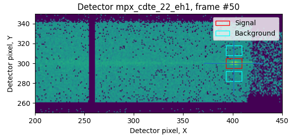On this image shadow from slits, detector gaps and ROIs can be clearly seen.

Intensity integration

Let’s integrate the intensity in ROIs and plot it together:

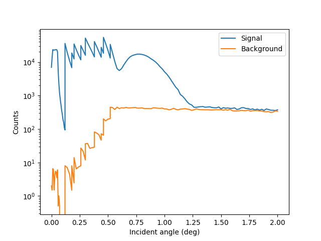
This picture is as expected and highlights the importance of background subtraction. Here, starting from ca. 1.25 degrees of incident angle, it is difficult to distinguish between signal and the background. Thanks to the use of a 2D detector, it is possible to measure both background and signal at the same time.

Subtract the background

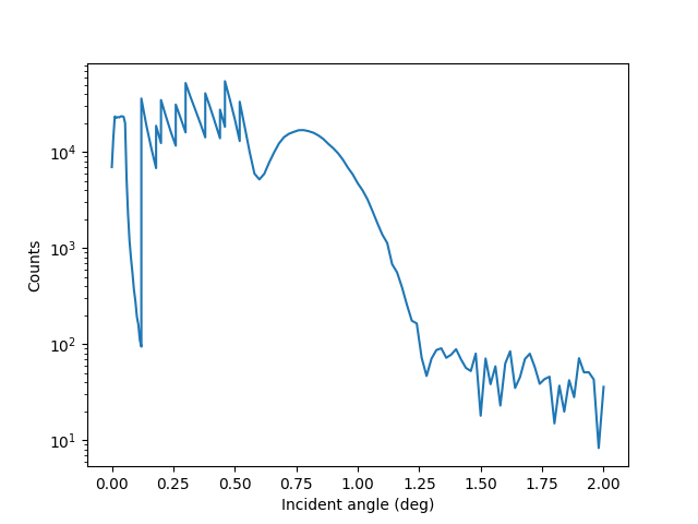
Background subtraction reveals a hint to a second fringe, but to obtain reflectivity we need to normalize by the filter transmission.

Normalize by filter transmission

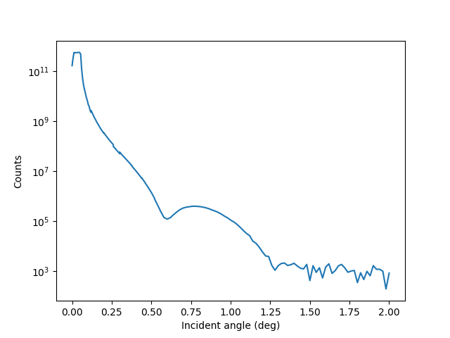
This resembles reflectivity, however, a few things are off: x-axis is still in angles and is energy-dependent, there are intensity steps during filter change, and reflectivity is in arbitrary units.

Convert angles to q

Using a formula for $q_z$:

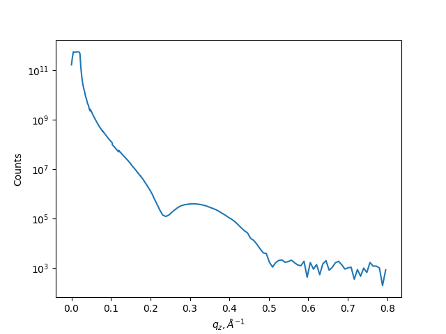
Correct intensity steps using double points

To get rid of the intensity jumps we go through all the filter changes and compare the intensity with a “new” and “old” filter. This ratio is used to extract “true” transmission ratio between the filters, assuming that sample does not change. This allows to obtain a smooth reflectivity curve.

Intensity normalization

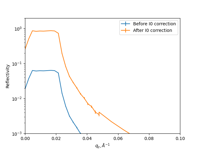
Because the first part of the reflectivity (up to $ 2 \alpha_c $) was measured with the same filter as z-scan, preceding it, we can extract precise value of the intensity. It allows for a correct normalization of intensity, so that $ R(q<q_c) =1 $.

Footprint correction

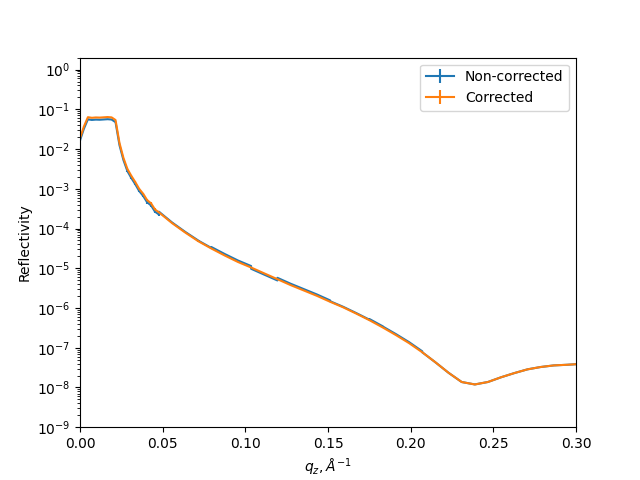
Due to the small grazing angle, footprint of the beam on sample is significantly increased. This means that for small samples it can be larger than the sample size. While for liquid surfaces it is less of a concern, for small solid sample it may have a significant effect. Let’s estimate the footprint of the typical ID10 beam ($b_V = 20 $ microns, 22.5 keV) at critical angle for Si.

\(\alpha_c = 0.07923^{\mathrm{o}} = 0.00138\,\mathrm{rad}\) \(d_c = \frac{b_V}{\sin \alpha_c} = \frac{20 \cdot 10^{-6} }{\sin\alpha_c \simeq \alpha_c \simeq 0.00138} = 0.0144\,\mathrm{m} = 1.44\,\mathrm{cm}\)

Therefore, samples, that are larger than 1.44 cm should be fully illuminated at critical angle. Langmuir through size is 17 cm, so only very small angles are affected by this correction for experiments on liquds. Nevertheless, the effect of this correction is visible.

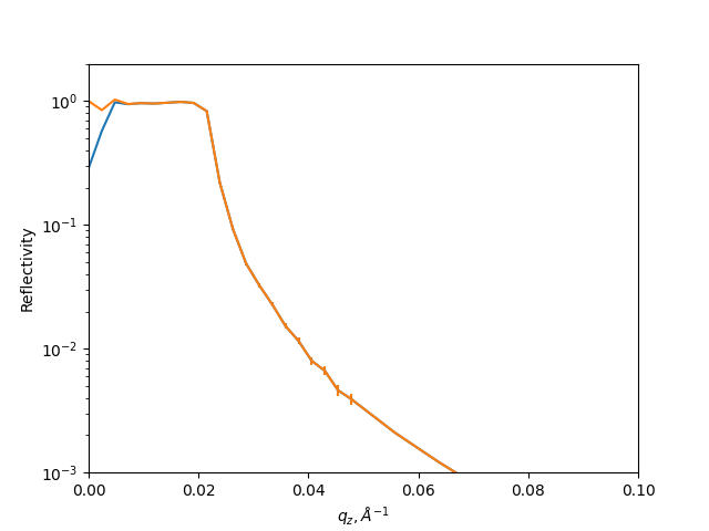
After this step reflectivity curve is fully corrected and can be used for fitting. All these steps are included in auto-correction procedure, implemented in the library.

Grazing Incidence Diffraction